Seeing a turbine tire
A wind turbine that loses two percent of its output, or that drops to half power now and then, can run for months before anyone notices. The standard check compares averages. Many faults change the shape of the data instead.
Born from the forecast
On November 5, 2026 Singularity registered, with a fingerprint, that the Wasserstein distance — a way of measuring how far one distribution must move to become another, born in the mathematics of transporting earth — would enter energy engineering, a subfield where no work used it yet. It was one of the “classic and unexpected” forecasts: an old method, a field where nobody uses it. We checked whether anyone had applied it to power-curve monitoring and found nothing, so we ran the test ourselves.
What we found
How we tested it
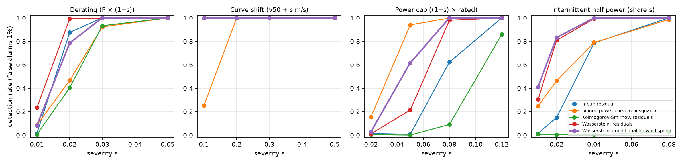
A simulated turbine, four weeks of healthy reference, one-week test windows, a false-alarm rate fixed at 1%. Four kinds of fault, four severities each, five detectors — all written down before the single run. The results are reported as they came, including the case where the old method wins.
Why it matters
The conditional Wasserstein distance uses the same bins and the same reference as the usual power curve, so it can be added to an existing monitor at no cost. Next step: real SCADA data with logged faults.
The paper
Wasserstein distances for wind-turbine power-curve monitoring: a pre-specified simulation comparison
· November 2026 · preprint
Abstract
Wind-turbine performance monitoring compares recent SCADA records with a healthy reference, usually through a binned power curve or a residual statistic. These tools compare means; many faults instead change the shape of the distribution of power at a given wind speed. We compare five detectors on simulated 10-minute SCADA data with a fixed false-alarm rate of 1% per one-week window: the mean residual, a binned power-curve chi-square statistic, the Kolmogorov–Smirnov statistic on residuals, the 1-Wasserstein distance between residual distributions, and a 1-Wasserstein distance conditional on wind speed. Four fault families at four severities were specified before the single run. Averaged over the twelve non-trivial scenarios, detection rates were 73% (conditional Wasserstein), 71% (residual Wasserstein), 67% (binned chi-square), 54% (mean residual) and 28% (Kolmogorov–Smirnov). The Wasserstein detectors were best for derating and intermittent faults, while the binned chi-square was clearly best for a power cap. No detector dominates; the conditional Wasserstein distance is the best single choice in this benchmark and costs no more than a binned power curve.
| detector | derating | power cap | intermittent | mean of 12 |
|---|---|---|---|---|
| mean residual | 0.72 | 0.41 | 0.49 | 0.54 |
| binned chi-square | 0.62 | 0.77 | 0.62 | 0.67 |
| Kolmogorov–Smirnov | 0.58 | 0.24 | 0.01 | 0.28 |
| Wasserstein, residuals | 0.81 | 0.55 | 0.78 | 0.71 |
| Wasserstein, conditional | 0.72 | 0.66 | 0.81 | 0.73 |
Mean detection rate over four severities. A shift of the power curve is detected by every statistic from the smallest severity tested, except the binned chi-square at 0.1 m/s (25%), and is left out of the mean.
Limitations
Simulated data, independent records, stationary wind climate; real SCADA data have autocorrelation, air-density seasons, wakes and gaps, which call for block-bootstrap thresholds. The fault list is short and the severities were chosen by us.